In the 68th edition of the Wrong Read, Blair Andrews uses a random forest to help you find the most important metrics for wide receiver evaluation.

A couple of years ago, I did a fun study called the Ultimate WR Prospect Metrics Guide to determine which metrics best correlated with NFL success. That was a good first step, but it had a couple of holes. First, it didn’t examine any physical measurements. Second, it assumed linear relationships for all the metrics involved. That’s not always the case. The study on WR hand size in the Wrong Read, No. 61 is a good example.

Non-Linearity and Regression Trees

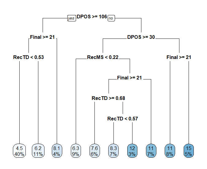
With those things in mind, perhaps we can find a better way to determine which WR prospect metrics we should be paying the closest attention to. Dave Caban recently undertook a similar study using a regression tree. The great thing about regression trees is that they don’t assume variables have a linear relationship with whatever you’re trying to predict. And they make this fact easy to understand by translating each variable into a threshold for success.

In Dave’s regression tree, draft position is the most important variable. But rather than giving an equation for turning draft position into a projection, the regression tree tells us that WRs drafted in the top 105 picks tend to have greater success.

Intuitively, this makes sense — a WR picked at the end of the third round should probably not be viewed as a significantly worse asset compared to one picked at the end of the second round. But there’s a big difference between being a third-round WR and a sixth-round WR.

Later we see another split on draft position, with players picked in the top-30 going on to even greater success. This also makes some sense, as first-round WRs often get the most early opportunity. With these two splits, you divide the draft almost perfectly into three distinct sections: Day 1, Day 2, and Day 3. In other words, even draft position doesn’t appear to be linear.

Building on Regression Trees

The regression tree helps us understand the interaction between different variables and what it is you want to predict. And we can even go further. What if instead of growing one tree, we grow 500 trees, each with a random subset of the data and a random subset of the variables? This technique is called, fittingly, a random forest. It lets us better isolate different variables to reduce noise, and it also enables us to include more variables in our results.

There are some trade-offs. What you gain in robustness and comprehensiveness, you lose in interpretability. Because we’re growing 500 trees, we can’t visualize just one as a representative sample. However, we can easily use a random forest model to measure relative variable importance.

There are many ways to measure variable importance, but one of my favorite ways — and one of the most intuitive ways — is to use a permutation method. The method gets its name because you measure variable importance by randomly shuffling each variables’ values and seeing what effect that has on overall model accuracy. If replacing actual values with random values has a negligible effect, that means the variable isn’t very important. A large negative effect means the variable is important.^[1]If it has a large positive effect, that would imply that random values give you a more accurate picture than the actual values, which makes little sense. This doesn’t mean the actual values are actively misleading. Rather, in effect this means that the actual values might as well be random, so an increase in model accuracy — a decrease in mean squared error — amounts to the same as no change. We can do this multiple times to find the average decrease in model accuracy for each metric, which gives us a robust and illuminating ranking of variable importance.

What Are the Most Important WR Metrics?

The chart below measures relative importance in terms of the increase in mean squared error after random shuffling. In other words, how much error do random values add to the overall model compared to actual values? Higher numbers indicate that we lose more accuracy with random values. So higher numbers are better.